Optimization of a Constrained Quadratic Function

Charles HAMAKER
Department of Mathematics and Computer Science
PO Box 3517 Saint Mary’s College of California,
Moraga, CA,94575
chamaker@stmarys-ca.edu

Dedicated on the occasion of his 60th birthday to Neculai Andrei in appreciation of a lifetime of contributions to mathematics, as a productive researcher, an author of valuable texts and software, and a leader in the mathematical community.

Abstract: For A a positive definite, symmetric n x n matrix and b a real n-vector, the objective function is optimized over the unit sphere. The proposed iterative methods, based on the gradient of f, converge in general for maximization and for large |b| for minimization with the principal computational cost being one or two matrix-vector multiplications per iteration. The rate of convergence improves as |b| increases, becoming computationally competitive in that case with algorithms developed for the more general problem wherein A may be indefinite.

Keywords: Constrained optimization, quadratic functions, iterated gradients, acceleration of convergence.

Charles Hamaker works in applicable analysis, particularly the application of Radon transforms to mathematical tomography and differential equations. He is also the director of his college’s core undergraduate program in reading classical texts of western culture.

>>Full text
CITE THIS PAPER AS:
Charles HAMAKER, Optimization of a Constrained Quadratic Function, Studies in Informatics and Control, ISSN 1220-1766, vol. 18 (1), pp. 21-32, 2009.

1. Introduction and Preliminaries

Let A be a real-valued, positive definite, symmetric n x n matrix, and let b be a real-valued n-vector. The problem under consideration here is:

Optimize over .

For small dimensions, the well-established approach involving diagonalization of A, outlined in [Golub and Van Loan 1996] and sketched in the remark preceding Lemma 1, suffices for both maximization and minimization. For large dimensions, the computational cost of diagonalization is excessive.

The maximization problem was encountered for n=4 in computations for lattice gauge simulations [Montero, 1999]. With A allowed to be indefinite, the minimization problem is the trust region subproblem which must be solved in each iteration of a trust region method [Conn, Gould, Toint, 2000] and [Hager, 2001]. The subproblem has been the subject of considerable attention, resulting in sophisticated iterative algorithms (see [Hager, 2001], [Sorenson, 1997], and [Rendl and Wolkowicz, 1997]). For instance, the SSM algorithm described in [Hager, 2001] converges quadratically, using the Lanczos process for startup and with each iterate being the solution of the problem on a low-dimensional subspace. That subspace is determined in part by applying Newton’s method at the previous iterate to the associated Lagrange problem. As is typical of these algorithms, the tradeoff for the small number of iterations required is that initialization and each iteration require a significant number of matrix-vector multiplications. See [Hager, 2001] for a comparison of the computational effectiveness of some of these algorithms. These minimization algorithms are adaptable to the maximization problem presumably with similar computational cost.

Denoting the eigenvalues of A by , direct the corresponding orthonormal basis of eigenvectors so that

and in the case that , so that

and let E denote the orthogonal matrix having the as columns. Then, since the change of coordinates diagonalizes A and preserves the constraint set , it can be observed that

Thus, with respect to the coordinates , the problem takes the diagonalized form:

Optimize over where and are as above.

It is convenient to adopt the following notations. For , representation in coordinates will be with respect to the orthonormal eigenbasis and will be denoted by . The outer subscript will be omitted when no ambiguity results, e.g. while . The euclidean norm of a vector x will be denoted by |x|. The subset of consisting of all vectors with non-negative (non-positive) coordinates will be denoted by .

Geometric insight into the problem follows from completing the square in the diagonalized form of to obtain

where

Thus, for c>-k, the level hypersurface f(x) = c is an ellipsoid with center at .

It is the simplicity of this geometric characterization that suggests the iterative algorithm for the maximization problem: where T(x) is the normalization of the gradient. Note that the solution is a fixed point for T. While convergence in general will be established, it is reasonable to expect that the rate will improve as |b| increases, moving the common center of the ellipsoids further from the origin and thus resulting in less variation of over the constraint set . The algorithm for the minimization problem (See section 4) is based on similar heuristic considerations.

Characterization of the maximizing vector can begin by observing in the diagonalized form of the problem that it must have non-negative coordinates because the are positive, and furthermore must satisfy the Lagrange multiplier condition:

for some (1)

Since , this implies

(2)

This leads to defining

and observing that the requirement that means that μ must satisfy the secular equation g(t)=1.

If b₁>0, then the requirement that implies that , and hence that all the are defined by (2). Because g(t) is unbounded and decreasing on and approaches 0 as , there exists a unique satisfying . Thus there is a unique maximizing point w.

In the case that and , the requirement that implies , and there is a unique satisfying . Then (2) can be satisfied for i < k in one of two ways. First, if , then . Second, if and (in which case ) the unit vectors determined by the Lagrange condition have coordinates determined by (2) for , while . Thus , where

For the unit vector determined by in (2),, and is positive for . Thus the desired maximum corresponds to the largest value of μ satisfying (1), namely the larger of and .

Remark: Assuming that the problem has been diagonalized, i.e. the eigenvectors have been found, and that , μ in equation (1) can be found by solving the secular equation g(t)=1 and then used in equation (2) to find w. This approach is outlined in [Golub and Van Loan, 1996] for the minimization problem and used in [Montero, 1999] to solve the maximization problem for n = 4.

The resulting characterization of the maximizing vector is summarized as follows.

Lemma 1

1. If , then the maximizing vector w satisfies and the corresponding Lagrange multiplier satisfies .

2. If and , then and .

3. If and , then with the set S of maximizing vectors consisting of all w with determined by (2) for and satisfying .

Characterization of the minimizing vector v as corresponding via (2) to the smallest value which satisfies (1) is completely similar, and is given in Lemma 2.2 of [Hager 2001]. In that paper, the counterparts to cases 1, 2, and 3. are referred to as non-degenerate, non-degenerate degenerate, and degenerate, and the literature on the trust region subproblem refers to cases 2 and 3 collectively as the hard case.

It is useful to characterize the optimizing vectors and their multipliers for |b| large.

Lemma 2 For , let b= τ u, τ > 0. Then, for fixed A,

1. and .

2. and

Proof: The secular equation g(t) = 1 becomes

To establish case 1, note first that µ_o, the largest solution of the secular equation, satisfies . Thus for τ large enough,, and so . Setting t = μ in the secular equation, multiplying by , and taking limits gives

Then

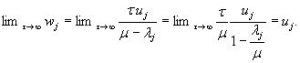
Case 2 is established similarly.

REFERENCES:

Akers, W. and D. Camp, Kinetics of the methane-steam reaction, AIChE Journal, 1 (1955), pp. 471–475.
Allen, D., E. Gerhard, and M. Likins Jr, Kinetics of the methane-steam reaction, Industrial & Engineering Chemistry Process Design and Development, 14 (1975), pp. 256–259.
Belke, J., Chemical Accident Risks in US Industry a Preliminary Analysis of Accident Risk Data from US Hazardous Chemical Facilitieso, United States Environmental Protection Agency, Chemical Emergency Preparedness and Prevention Office, Washington, D.C., 2000.
Bodrov, N., L. Apel’baum, and M. Tempkin, Kinetics of the reaction of methane with water vapour catalysed by nickel on a porous carrier, Kinetika L Kataliz, 8 (1967), pp. 821–828.
R. Dubes, The theory of applied probability, Prentice-Hall, 1968.
Fogel, E. and Y. Huang, Value of Information in System Identification-Bounded Noise Case., Automatica, 18 (1982), pp. 229–238.
Hammersley,J., D. Handscomb, Monte Carlo methods, Methuen, 1964.
Hastie, T., R. Tibshirani, and J. Friedman, The Elements of Statistical Learning: Data Mining, Inference, and Prediction, Springer, Berlin, 2001.
Helfferich, F., Kinetics of Homogeneous Multistep Reactions, Elsevier Science, 2001.
Jacod, J. and P. Protter, Probability Essentials, Springer, Berlin, 2003.
Juang, J. and R. Pappa, Eigensystem realization algorithm for modal parameter identification and model reduction., Journal of Guidance, Control, and Dynamics, 8 (1985), pp. 620–627.
Marek, L. F. and D.A. Hahn, Catalytic Oxidation of Organic Compounds in the Vapor Phase, A. C. S. Monograph 61, Chemical Catalog Co., New York, 1932.
McQuarrie, D.A. and J.D. Simon, Physical Chemistry: A Molecular Approach, University Science Books, 1997.
Moe, J. and E. Gerhard, Chemical reaction and heat transfer rates in the steam methane reaction, in AIChE Symposium, 56th National Meeting, San Francisco, Calif., May, 1965.
Niederreiter, H., Random number generation and quasi-Monte Carlo methods, Society for Industrial and Applied Mathematics, Philadelphia, 1992.
Norton, J., Identification of parameter bounds for ARMAX models from records with bounded noise, International Journal of Control, 45 (1987), pp. 375–390.
Ragan, P., M. Kilburn, S. Roberts, and N. Kimmerle, Chemical plant safety- applying the tools of the trade to a new risk, Chemical Engineering Progress, 98 (2002), pp. 62–68.
Rubinstein, R., Simulation and the Monte Carlo Method, John Wiley & Sons, Inc., New York, NY, USA, 1981.
Ruscic, B., Active Thermochemical Tables, Yearbook of Science and Technology (annual update volume to: McGraw-Hill Encyclopedia of Science and Technology), McGraw-Hill, New York City, 2004.
Ruscic, B. R.E. Pinzon, M.L. Morton, N.K. Srinivasan, M.-C. Su, J.W. Sutherland, and J.V. Michael, Active thermochemical tables: Accurate enthalpy of formation of hydroperoxyl radical, HO2, J. Phys. Chem. A, 110 (2006), pp. 6592–6601.
Ruscic, B., R.E. Pinzon, M.L. Morton, G.von Laszewski, S. Bittner, S.G. Nijsure, K.A. Amin, M.Minkoff, and A.F. Wagner, Introduction to active thermochemical tables: Several “key” enthalpies of formation revisited, J. Phys. Chem. A, 108 (2004), pp. 9979–9997.
Ruscic, B., R.E. Pinzon, G.von Laszewski, D. Kodeboyina, A. Burcat, D. Leahy, D. Montoya, A. Wagner, Active thermochemical tables: Thermochemistry for the 21st century, J. Phys. Conf. Ser., 16 (2005), pp. 561–570.
Sabatier, P., Catalysis in organic chemistry, Van Nostrand, New York, 1922.
Silberberg, M., R. Duran, C. Haas, and A. Norman, Chemistry: The Molecular Nature of Matter and Change, McGraw-Hill, 2006.
Singh, C., and D. Saraf, Simulation of side-fired steam-hydrocarbon reformers, Ind. Eng. Chem. Process Des. Dev., 18 (1979), pp. 1–7.
Sloan, I.H., and S. Joe, Lattice methods for multiple integration, The Clarendon Press Oxford University Press, New York, 1994.
Smith, J., H. Van Ness, and M. Abbott, Introduction to Chemical Engineering Thermodynamics, McGraw-Hill Science / Engineering/ Math, 2004.
Sprott, J., Chaos and Time-Series Analysis, Oxford University Press, 2003.
Therrien, C., and M. Tummala, Probability for Electrical and Computer Engineers, CRC Press, 2004.
Van Hook, J., Methane-steam reforming, Catalysis Reviews of Science Engineering, 21 (1980).
Wackerly, D., W. Mendenhall, and R. Scheaffer, Mathematical statistics with applications, Duxbury Pacific Grove, CA, 2002.